Modern Recurrent Neural Network
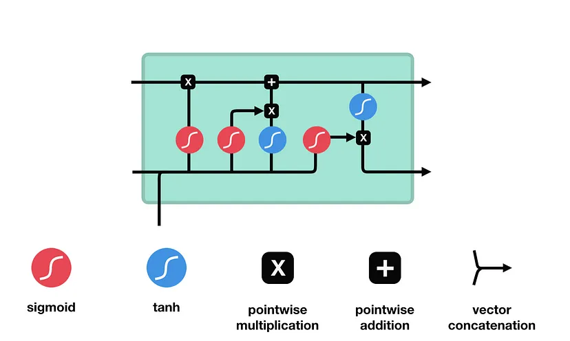
I. Long Short Term Memory (LSTM)
Long Short Term Memory networks – usually just called “LSTM” – are a special kind of RNN, capable of learning long-term dependencies. LSTM are explicitly designed to avoid the short-term dependency problem. Remembering information for long periods of time is practically their default behavior, not something they struggle to learn!
Step-by-Step LSTM Walk Through
Forget gate
First step decides what information should be thrown away or kept. Information from the previous hidden state and information from the current input is passed through the sigmoid function. Values come out between 0 and 1. The closer to 0 means to forget, and the closer to 1 means to keep:
\[f_{t} = \sigma (W_{f} \cdot [h_{t-1},x_{t}] + b_{f}) \tag{1}\]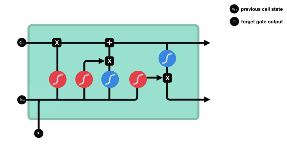
Input gate
The next step is to decide what new information will be updated in the cell state. First, pass the previous hidden state and current input into a sigmoid layer called the “input gate layer”. That decides which values will be updated by transforming the values to be between 0 and 1. 0 means not important, and 1 means important. The hidden state and current input also be passed into the tanh function to squish values between -1 and 1 to help regulate the network and creates new candidate values, $\tilde C_{t}$:
\[i_{t} = \sigma (W_{i} \cdot [h_{t-1},x_{t}] + b_{i}) \tag{2}\] \[\tilde C_{t} = \tanh(W_{C} \cdot [h_{t-1},x_{t}] +b_{C}) \tag{3}\]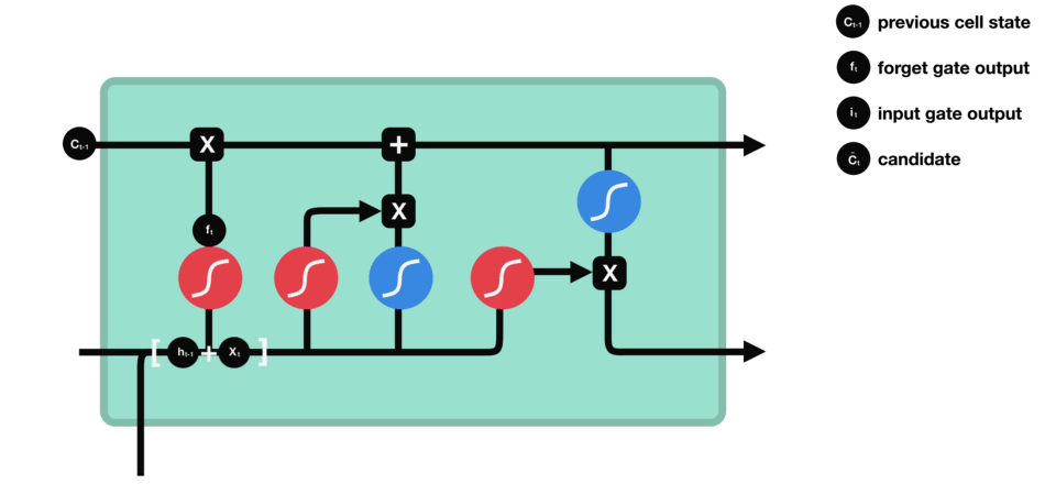
Cell state
Now we have enough infomation to update the new cell state. We multiply the old state by $f_{t}$, forgetting the things we decided to forget earlier. Then we add $i_{t} \ast \tilde C_{t}$. This is the new candidate values, scaled by how much we decided to update each state value:
\[C_{t} = f_{t} \ast C_{t-1} + i_{t} \ast \tilde C_{t} \tag{4}\]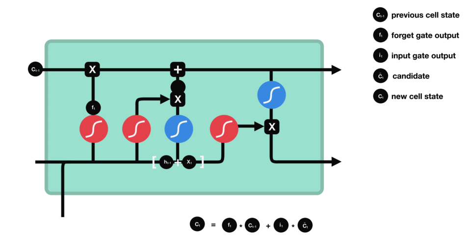
Output gate
Last we have the output gate. The output gate decides what the next hidden state should be. Remember that the hidden state contains information on previous inputs. The hidden state is also used for predictions. First, we run a sigmoid layer which decides what parts of the cell state we’re going to output. Then, we put the cell state through tanh and multiply it by the output of the sigmoid gate, so that we only output the parts we decided to:
\[o_{t} = \sigma (W_{o} \cdot [h_{t-1},x_{t}] + b_{o}) \tag{5}\] \[h_{t} = o_{t} \ast \tanh(C_{t}) \tag{6}\]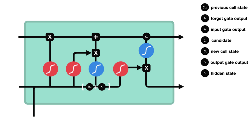
Code:
1
2
3
4
5
6
7
8
9
10
11
12
13
14
15
def lstm(inputs, state, params):
    [W_xi, W_hi, b_i, W_xf, W_hf, b_f, W_xo, W_ho, b_o, W_xc, W_hc, b_c,
    W_hq, b_q] = params
    (H, C) = state
    outputs = []
    for X in inputs:
        I = torch.sigmoid((X @ W_xi) + (H @ W_hi) + b_i)
        F = torch.sigmoid((X @ W_xf) + (H @ W_hf) + b_f)
        O = torch.sigmoid((X @ W_xo) + (H @ W_ho) + b_o)
        C_tilda = torch.tanh((X @ W_xc) + (H @ W_hc) + b_c)
        C = F * C + I * C_tilda
        H = O * torch.tanh(C)
        Y = (H @ W_hq) + b_q
        outputs.append(Y)
    return torch.cat(outputs, dim=0), (H, C)
II. Gated Recurrent Unit (GRU)
GRU is the variation of the LSTM. It combines the forget and input gates into a single “update gate.” It also merges the cell state and hidden state, and makes some other changes.
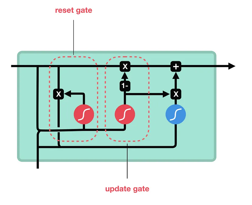
Update gate
The update gate acts similar to the forget and input gate of an LSTM. It decides what information to throw away and what new information to add.
\[z_{t} = \sigma (W_{z} \cdot [h_{t-1},x_{t}] + b_{z}) \tag{7}\]Reset gate
The reset gate would allow us to control how much of the previous state we might still want to remember:
\[r_{t} = \sigma (W_{r} \cdot [h_{t-1},x_{t}] + b_{r}) \tag{8}\]Candidate Hidden State
Influence of the previous states can be reduced with the elementwise multiplication of $r_{t}$ and $h_{t−1}$. Whenever the entries in the reset gate $r_{t}$ are close to 1, we recover a vanilla RNN. For all entries of the reset gate $r_{t}$ that are close to 0, the candidate hidden state is the result of an MLP with Xt as the input. Any pre-existing hidden state is thus reset to defaults. Then we use a nonlinearity in the form of tanh to ensure that the values in the candidate hidden state remain in the interval (−1, 1):
\[\tilde h_{t} = \tanh(W \cdot [r_{t} \ast h_{t-1},x_{t}]) \tag{9}\]Hidden State
The update gate $z_{t}$ determines the extent to which the new hidden state $h_{t}$ is just the old state $h_{t-1}$ and by how much the new candidate state $\tilde h_{t}$ is used. The update gate Zt can be used for this purpose, simply by taking elementwise convex combinations between both $h_{t-1}$ and $\tilde h_{t}$. This leads to the final update equation for the GRU:
\[h_{t} = z_{t} \odot h_{t-1} + (1 - z_{t}) \odot \tilde h\_{t} \tag{10}\]In summary, GRUs have the following two distinguishing features:
- Reset gates help capture short-term dependencies in sequences.
- Update gates help capture long-term dependencies in sequences.
Code:
1
2
3
4
5
6
7
8
9
10
11
12
def gru(inputs, state, params):
    W_xz, W_hz, b_z, W_xr, W_hr, b_r, W_xh, W_hh, b_h, W_hq, b_q = params
    H, = state
    outputs = []
    for X in inputs:
        Z = torch.sigmoid((X @ W_xz) + (H @ W_hz) + b_z)
        R = torch.sigmoid((X @ W_xr) + (H @ W_hr) + b_r)
        H_tilda = torch.tanh((X @ W_xh) + ((R * H) @ W_hh) + b_h)
        H = Z * H + (1 - Z) * H_tilda
        Y = H @ W_hq + b_q
        outputs.append(Y)
    return torch.cat(outputs, dim=0), (H,)