Proximal Policy Optimization

Proximal Policy Optimization (PPO) is a popular reinforcement learning algorithm used for training policies in reinforcement learning tasks. It was introduced by OpenAI in 2017 and has since gained significant attention due to its simplicity and effectiveness.
I will briefly discuss the main points of policy gradient methods and Proximal Policy Optimization (PPO).
I. Vanilla Policy Gradient
In the context of RL, a policy $\pi$ is simply a function that returns a feasible action a given a state s. In policy-based methods, the function (e.g., a neural network) is defined by a set of tunable parameters $\theta$. We can adjust these parameters, observe the differences in resulting rewards, and update $\theta$ in the direction that yields higher rewards. This mechanism underlies the notion of all policy gradient methods.
The simplest way is to combine the policy and the reward into one objective function. We can express this objective function dependent on $\theta$:
\[J(\theta) = \sum_{a \in \mathcal{A}} \pi_\theta(a \vert s) R^\pi(s, a)\]To determine the update direction that improve the objective function, policy gradient methods rely on gradients ∇_θ (gradient ascend). This yields the following update function:
\[\theta \leftarrow \theta + \Delta J(\theta)\]The Log-Derivative Trick: The log-derivative trick is based on a simple rule from calculus: the derivative of \log x with respect to x is 1/x. When rearranged and combined with chain rule, we get:
\[\nabla_{\theta} P(\tau | \theta) = P(\tau | \theta) \nabla_{\theta} \log P(\tau | \theta).\]The Advantage Estimation: the advantage of an action, describes how much better or worse it is than other actions on average (relative to the current policy):
\[A^{\pi}(s_t,a_t) = Q^{\pi}(s_t,a_t) - V^{\pi}(s_t)\]Policy Gradient: Let $\pi_{\theta}$ denote a policy with parameters $\theta$, and $J(\pi_{\theta})$ denote the expected finite-horizon undiscounted return of the policy. The gradient of $J(\pi_{\theta})$ is:
\[\nabla_{\theta} J(\pi_{\theta}) = {E}_{\tau \sim \pi_{\theta}}{ \sum_{t=0}^{T} \nabla_{\theta} \log \pi_{\theta}(a_t|s_t) A^{\pi_{\theta}}(s_t,a_t)},\]where $\tau$ is a trajectory and $A^{\pi_{\theta}}$ is the advantage function for the current policy.
The policy gradient algorithm works by updating policy parameters via stochastic gradient ascent on policy performance:
\[\theta_{k+1} = \theta_k + \alpha \nabla_{\theta} J(\pi_{\theta_k})\]Policy gradients suffers from major drawbacks:
- Sample inefficiency — Samples are only used once. After that, the policy is updated and the new policy is used to sample another trajectory. As sampling is often expensive, this can be prohibitive. However, after a large policy update, the old samples are simply no longer representative.
- Inconsistent policy updates — Policy updates tend to overshoot and miss the reward peak, or stall prematurely. Especially in neural network architectures, vanishing and exploding gradients are a severe problem. The algorithm may not recover from a poor update.
- High reward variance — Policy gradient is a Monte Carlo learning approach, taking into account the full reward trajectory (i.e., a full episode). Such trajectories often suffer from high variance, hampering convergence. [This issue can be addressed by adding a critic, which is outside of the article’s scope]
II. Proximal Policy Optimization (PPO)
The idea with PPO is that we want to improve the training stability of the policy by limiting the change you make to the policy at each training epoch: we want to avoid having too large policy updates.
There are two reasons:
- Smaller policy updates during training are more likely to converge to an optimal solution.
- A too big step in a policy update can result in falling “off the cliff” (getting a bad policy) and having a long time or even no possibility to recover.
So with PPO, we update the policy conservatively. To do so, we need to measure how much the current policy changed compared to the former one using a ratio calculation between the current and former policy. And we clip this ratio in a range $[1-\epsilon,1+\epsilon]$ meaning that we remove the incentive for the current policy to go too far from the old one (hence the proximal policy term).
1. PPO Formula
Let’s denote the ratios between the new the old policies:
\[r(\theta) = \frac{\pi_\theta(a \vert s)}{\pi_{\theta_\text{old}}(a \vert s)}\]We have the objective function:
\[J^\text{CLIP} (\theta) = \mathbb{E} [ \min( r(\theta) \hat{A}_{\theta_\text{old}}(s, a), \text{clip}(r(\theta), 1 - \epsilon, 1 + \epsilon) \hat{A}_{\theta_\text{old}}(s, a))]\]where:
$\theta$: is the policy parameters.
$E$: denotes the empirical expectation over timesteps.
$r(\theta)$: the ratio of the probability under the new and old policies, respectively.
A: the estimated advantage.
$\epsilon$: the hyperparameter used to clip the ratios $r(\theta)$.
2. Clipped Surrogate Objective Function
Let’s see what this Clipped Surrogate Objective Function looks like:
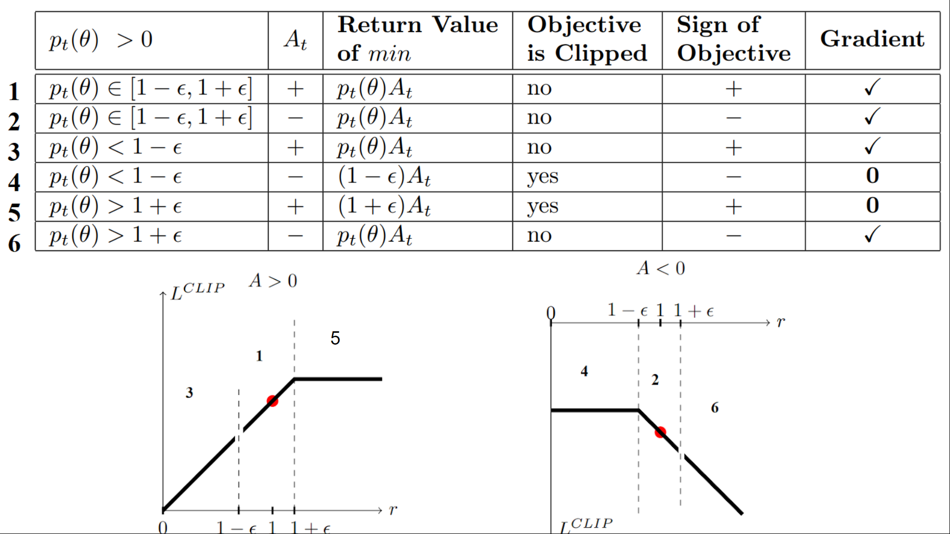
Advantage is positive: Suppose the advantage for that state-action pair is positive, in which case its contribution to the objective reduces to
\[J= \min\left( \frac{\pi_{\theta}(a|s)}{\pi_{\theta_k}(a|s)}, (1 + \epsilon) \right) A^{\pi_{\theta_k}}(s,a).\]Because the advantage is positive, the objective will increase if the action becomes more likely-that is, if $\pi_{\theta}(a|s)$ increases. But the min in this term puts a limit to how much the objective can increase. Once $\pi_{\theta}(a|s)>(1+\epsilon)\pi_{\theta_k}(a|s)$ , the min kicks in and this term hits a ceiling of $(1+\epsilon)A^{\pi_{\theta_k}}(s,a)$ . Thus: the new policy does not benefit by going far away from the old policy.
Advantage is negative: Suppose the advantage for that state-action pair is negative, in which case its contribution to the objective reduces to
\[J = \max\left( \frac{\pi_{\theta}(a|s)}{\pi_{\theta_k}(a|s)}, (1 - \epsilon) \right) A^{\pi_{\theta_k}}(s,a).\]Because the advantage is negative, the objective will increase if the action becomes less likely—that is, if $\pi_{\theta}(a|s)$ decreases. But the max in this term puts a limit to how much the objective can increase. Once $\pi_{\theta}(a|s)<(1-\epsilon)\pi_{\theta_k}(a|s)$ , the max kicks in and this term hits a ceiling of $(1-\epsilon)A^{\pi_{\theta_k}}(s,a)$ . Thus, again: the new policy does not benefit by going far away from the old policy.
3.Code
Here are a simple code of the PPO’s loss function:
1
2
3
4
5
6
7
8
9
10
11
def PPOLoss(self,value,value_new,entropy,log_prob,log_prob_new,rtgs):
    advantage             = rtgs - value.detach()
    advantage             = (advantage - advantage.mean()) / (advantage.std()+1e-8)
    ratios                = torch.exp(torch.clamp(log_prob_new-log_prob.detach(),min=-1000.,max=20.))
    weighted_prob         = ratios * advantage
    weighted_clipped_prob = torch.clamp(ratios,1-0.2,1+0.2) * advantage
    actor_loss            = -torch.min(weighted_prob,weighted_clipped_prob)
    value_clipped         = value + torch.clamp(value_new - value, -0.2, 0.2)
    critic_loss           = 0.5 * torch.max((rtgs-value_new)**2,(rtgs-value_clipped)**2)
    total_loss            = actor_loss + self.critic_coef * critic_loss - self.entropy_coef * entropy
    return total_loss
III. Conclusion
Overall, Proximal Policy Optimization offers a robust and practical approach to reinforcement learning. Its simplicity, stability, and scalability make it a popular choice among researchers and practitioners alike, driving advancements in various fields such as robotics, game playing, and autonomous systems.