Transformer Variants
Although Transformers possess the potential to learn long-term dependencies, they face limitations in language modeling due to a fixed-length context. Additionally, in the context of Reinforcement Learning, where episodes can span thousands of steps and crucial observations for decision-making span the entire episode, traditional Transformers struggle to optimize effectively, often performing no better than a random policy. In this discussion, I will present several variants of Transformers designed to address these challenges and overcome these limitations.
Positional Encoding Variants
To begin, I will first examine the initial Positional Encoding in the vanilla Transformer model and its variant. Following that, I will explore various alternative versions of Transformer and their enhancements.
I. Positional Encoding (PE)
1.1 Absolute PE
Absolute PE describes the location or position of an entity in a sequence so that each position is assigned a unique representation.
The positional encoding outputs X+P using a positional embedding matrix $\mathbf{P} \in \mathbb{R}^{n \times d}$ of the same shape, whose element on the $i^{th}$ row and the ${(2j)}^{th}$ or the ${(2j+1)}^{th}$ column is:
1.2 Relative PE
1.2.1 Relation-aware Self-Attention
While absolute positional encodings work reasonably well, there have also been efforts to exploit pairwise, relative positional information. In Self-Attention with Relative Position Representations, Shaw et al. introduced a way of using pairwise distances as a way of creating positional encodings.
Relative positional information is supplied to the model on two levels: values and keys. This becomes apparent in the two modified self-attention equations shown below. First, relative positional information is supplied to the model as an additional component to the keys.
\[e_{ij} = \frac{x_i W^Q (x_j W^K + a_{ij}^K)^\top}{\sqrt{d_z}} \tag{2}\]The softmax operation remains unchanged from vanilla self-attention.
\[\alpha_{ij} = \frac{\text{exp} \space e_{ij}}{\sum_{k = 1}^n \text{exp} \space e_{ik}} \tag{3}\]Lastly, relative positional information is supplied again as a sub-component of the values matrix.
\[z_i = \sum_{j = 1}^n \alpha_{ij} (x_j W^V + a_{ij}^V) \tag{4}\]where $a_{ij}^{V},a_{ij}^{K} \in \mathbb{R}^{d}$ represent the edge between input elements $x_{i}$ and $x_{j}$.
In other words, instead of simply combining semantic embeddings with absolute positional ones, relative positional information is added to keys and values on the fly during attention calculation.
1.2.2 Efficient Implementation
For a sequence of length n and h attention heads, the space complexity of storing relative position representations can be reduced from $O(hn^{2}da)$ to $O(n^{2}da)$ by sharing them across each heads. Additionally, relative position representations can be shared across sequences. Therefore, the overall self-attention space complexity increases from $O(bhndz)$ to $O(bhndz + n^{2}da)$.
\[e_{ij} = \frac{x_i W^Q (x_j W^K) + x_i W^Q (a_{ij}^{K})^{T}}{\sqrt{d_z}} \tag{5}\]Transformer Variants
II. Transformer-XL
2.1 Vanilla Transformer
In vanilla transformer, the entire corpus is split into shorter segments of manageable sizes, and only train the model within each segment, ignoring all contextual information from previous segments. Under this training paradigm, information never flows across segments in either the forward or backward pass.
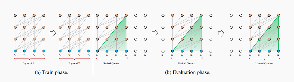
During evaluation, at each step, the vanilla model also consumes a segment of the same length as in training, but only makes one prediction at the last position. Then, at the next step, the segment is shifted to the right by only one position, and the new segment has to be processed all from scratch, which is extremely expensive.
2.2 Segment-Level Recurrence with State Reuse
To address the limitations of using a fixed-length context, a recurrence mechanism is introduced to the Transformer architecture.
During training, the hidden state sequence computed for the previous segment is fixed and cached to be reused as an extended context when the model processes the next new segment.Although the gradient still remains within a segment, this additional input allows the network to exploit information in the history, leading to an ability of modeling longer-term dependency and avoiding context fragmentation.
Formally, let the two consecutive segments of length L be $s_{\tau} = [x_{\tau,1},…,x_{\tau,L}]$ and $s_{\tau+1} = [x_{\tau+1,1},…,x_{\tau+1,L}]$ respectively. Denoting the n-th layer hidden state sequence produced fot the $\tau-th$ segment $s_{\tau}$ by $h_{\tau}^{n} \in {\mathbb{R}}^{L \times d}$, where d is the hidden dimension. Then, the n-th layer hidden state for segment $s_{\tau+1}$ is produced (schematically) as follows:
\[\tilde{h}_{\tau+1}^{n-1} = [SG(h_{\tau}^{n-1}) \circ h_{\tau+1}^{n-1}]\] \[{q}_{\tau+1}^{n}, {k}_{\tau+1}^{n}, {v}_{\tau+1}^{n} = {h}_{\tau+1}^{n-1} {W_{q}^{n}}^{T}, \tilde{h}_{\tau+1}^{n-1} W_{k}^{T}, \tilde{h}_{\tau+1}^{n-1} W_{v}^{T} \tag{6}\] \[h_{\tau+1}^{n} = TransformerBlock(q_{\tau+1}^{n},k_{\tau+1}^{n},v_{\tau+1}^{n})\]where:
- The function SG(·) stands for stop-gradient,
- The notation $[h_{u} \circ h_{v}]$ indicates the concatenation of two hidden sequences along the length dimension
- W denotes model parameters.
Compared to the standard Transformer, the critical difference lies in that the key $k_{n}^{\tau+1}$ and value $v_{\tau+1}^{n}$ are conditioned on the extended context $\tilde h_{\tau+1}^{n-1}$ and hence $h_{\tau}^{n-1}$ cached from the previous segment.
With this recurrence mechanism applied to every two consecutive segments of a corpus, it essentially creates a segment-level recurrence in the hidden states. As a result, the effective context being utilized can go way beyond just two segments. This additional connection increases the largest possible dependency linearly w.r.t. the number of layers as well as the segment length, i.e., O(N × L). Moreover, this recurrence mechanism also resolves the context fragmentation issue, providing necessary context for tokens in the front of a new segment.
2.3 Relative Positional Encoding
Naively applying segment-level recurrence does not work, however, because the positional encodings are not coherent when we reuse the previous segments. For example, consider an old segment with contextual positions [0, 1, 2, 3]. When a new segment is processed, we have positions [0, 1, 2, 3, 0, 1, 2, 3] for the two segments combined, where the semantics of each position id is incoherent through out the sequence.
In order to avoid this failure mode, the fundamental idea is to only encode the relative positional information in the hidden states. Conceptually, the positional encoding gives the model a temporal clue or “bias” about how information should be gathered, i.e., where to attend. For the same purpose, instead of incorporating bias statically into the initial embedding, one can inject the same information into the attention score of each layer. More importantly, it is more intuitive and generalizable to define the temporal bias in a relative manner.
Firstly, in the standard Transformer (Vaswani et al., 2017), the attention score between query $q_{i}$ and key vector $k_{j}$ within the same segment can be decomposed as
\[A_{i,j}^{abs} = \underbrace{E_{x_{i}}^{T} W_{q}^{T} W_{k} E_{x_{j}}}_{(a)} + \underbrace{E_{x_{i}}^{T} W_{q}^{T} W_{k} U_{j}}_{(b)} \tag{7}\] \[+ \underbrace{U_{i}^{T} W_{q}^{T} W_{k} E_{x_{j}}}_{(c)} + \underbrace{U_{i}^{T} W_{q}^{T} W_{k} U_{j}}_{(d)}\]where:
- E is the embedding inputs.
- U is the absolute positional embedding.
Following the idea of only relying on relative positional information:
\[A_{i,j}^{rel} = \underbrace{E_{x_{i}}^{T} W_{q}^{T} W_{k,E} E_{x_{j}}}_{(a)} + \underbrace{E_{x_{i}}^{T} W_{q}^{T} W_{k,R} R_{i-j}}_{(b)} \tag{8}\] \[+ \underbrace{u^{T} W_{k,E} E_{x_{j}}}_{(c)} + \underbrace{v^{T} W_{k,R} R_{i-j}}_{(d)}\]- The first change it make is to replace all appearances of the absolute positional embedding $U_{j}$ for computing key vectors in term (b) and (d) with its relative counterpart $R_{i−j}$ . This essentially reflects the prior that only the relative distance matters for where to attend. Note that R is a sinusoid encoding matrix without learnable parameters.
- Secondly, it introduce a trainable parameter $u \in R_{d}$ to replace the query $U_{i}^{T} W_{q}^T$ in term (c). In this case, since the query vector is the same for all query positions, it suggests that the attentive bias towards different words should remain the same regardless of the query position. With a similar reasoning, a trainable parameter $v \in R_{d}$ is added to substitute $U_{i}^{T} W_{q}^T$ in term (d).
- Finally, it deliberately separate the two weight matrices $W_{k,E}$ and $W_{k,R}$ for producing the content-based key vectors and location-based key vectors respectively.
Under the new parameterization, each term has an intuitive meaning:
- Term (a) represents content-based addressing.
- Term (b) captures a content-dependent positional bias.
- Term (c) governs a global content bias.
- Term (d) encodes a global positional bias.
Bonus: Efficient Computation of the Attention with Relative Positional Embedding
The naive way of computing the $W_{k,R}R_{i−j}$ for all pairs $(i, j)$ is subject to a quadratic cost. Author present a simple method with only a linear cost.
Define $Q$ in a reversed order, i.e., $Q_{k} = W_{k,R}R_{M+L−1−k}$. Firstly, notice that the relative distance $i − j$ can only be integer from $0$ to $M + L − 1$, where $M$ and $L$ are the memory length and segment length respectively. Hence, the rows of the matrix
\[\mathbf{Q}:=\left[\begin{array}{c} \mathbf{R}_{M+L-1}^{\top} \\ \mathbf{R}_{M+L-2}^{\top} \\ \vdots \\ \mathbf{R}_1^{\top} \\ \mathbf{R}_0^{\top} \end{array}\right] \mathbf{W}_{k, R}{ }^{\top}=\left[\begin{array}{c} {\left[\mathbf{W}_{k, R} \mathbf{R}_{M+L-1}\right]^{\top}} \\ {\left[\mathbf{W}_{k, R} \mathbf{R}_{M+L-2}\right]^{\top}} \\ \vdots \\ {\left[\mathbf{W}_{k, R} \mathbf{R}_1\right]^{\top}} \\ {\left[\mathbf{W}_{k, R} \mathbf{R}_0\right]^{\top}} \end{array}\right] \in \mathbb{R}^{(M+L) \times d}\]consist of all possible vector outputs of $W_{k,R}R_{i−j}$ for any $(i, j)$.
Next, collect the term $(b)$ for all possible $i, j$ into the following $L × (M + L)$ matrix:
\[\begin{aligned} & \mathbf{B}=\left[\begin{array}{cccccc} q_0^{\top} \mathbf{W}_{k, R} \mathbf{R}_M & \cdots & q_0^{\top} \mathbf{W}_{k, R} \mathbf{R}_0 & 0 & \cdots & 0 \\ q_1^{\top} \mathbf{W}_{k, R} \mathbf{R}_{M+1} & \cdots & q_1^{\top} \mathbf{W}_{k, R} \mathbf{R}_1 & q_1^{\top} \mathbf{W}_{k, R} \mathbf{R}_0 & \cdots & 0 \\ \vdots & \vdots & \vdots & \vdots & \ddots & \vdots \\ q_{L-1}^{\top} \mathbf{W}_{k, R} \mathbf{R}_{M+L-1} & \cdots & q_{L-1}^{\top} \mathbf{W}_{k, R} \mathbf{R}_{M+L-1} & q_{L-1}^{\top} \mathbf{W}_{k, R} \mathbf{R}_{L-1} & \cdots & q_{L-1}^{\top} \mathbf{W}_{k, R} \mathbf{R}_0 \end{array}\right] \\ & =\left[\begin{array}{cccccc} q_0^{\top} \mathbf{Q}_{L-1} & \cdots & q_0^{\top} \mathbf{Q}_{M+L-1} & 0 & \cdots & 0 \\ q_1^{\top} \mathbf{Q}_{L-2} & \cdots & q_1^{\top} \mathbf{Q}_{M+L-2} & q_1^{\top} \mathbf{Q}_{M+L-1} & \cdots & 0 \\ \vdots & \vdots & \ddots & \vdots & \ddots & \vdots \\ q_{L-1}^{\top} \mathbf{Q}_0 & \cdots & q_{L-1}^{\top} \mathbf{Q}_M & q_{L-1}^{\top} \mathbf{Q}_{M+1} & \cdots & q_{L-1}^{\top} \mathbf{Q}_{M+L-1} \end{array}\right] \\ & \end{aligned}\]Then, Author further define:
\[\widetilde{\mathbf{B}}=\mathbf{q Q}^{\top}=\left[\begin{array}{cccccc} q_0^{\top} \mathbf{Q}_0 & \cdots & q_0^{\top} \mathbf{Q}_M & q_0^{\top} \mathbf{Q}_{M+1} & \cdots & q_0^{\top} \mathbf{Q}_{M+L-1} \\ q_1^{\top} \mathbf{Q}_0 & \cdots & q_1^{\top} \mathbf{Q}_M & q_1^{\top} \mathbf{Q}_{M+1} & \cdots & q_1^{\top} \mathbf{Q}_{M+L-1} \\ \vdots & \vdots & \ddots & \vdots & \ddots & \vdots \\ q_{L-1}^{\top} \mathbf{Q}_0 & \cdots & q_{L-1}^{\top} \mathbf{Q}_M & q_{L-1}^{\top} \mathbf{Q}_{M+1} & \cdots & q_{L-1}^{\top} \mathbf{Q}_{M+L-1} \end{array}\right]\]It is easy to see an immediate relationship between $B$ and $\tilde B$, where the $i-th$ row of $B$ is simply a left-shifted of $i-th$ row of $\tilde B$ by $(L-i-1)$ column. Hence, the computation of $B$ only requires a matrix multiplication $qQ^{T}$ to compute $\tilde B$ and then a set of left-shifts.
Similarly, we can collect all term $(d)$ for all possible $i, j$ into another $L × (M + L)$ matrix $D$:
\[\mathbf{D}=\left[\begin{array}{cccccc} v^{\top} \mathbf{Q}_{L-1} & \cdots & v^{\top} \mathbf{Q}_{M+L-1} & 0 & \cdots & 0 \\ v^{\top} \mathbf{Q}_{L-2} & \cdots & v^{\top} \mathbf{Q}_{M+L-2} & v^{\top} \mathbf{Q}_{M+L-1} & \cdots & 0 \\ \vdots & \vdots & \ddots & \vdots & \ddots & \vdots \\ v^{\top} \mathbf{Q}_0 & \cdots & v^{\top} \mathbf{Q}_M & v^{\top} \mathbf{Q}_{M+1} & \cdots & v^{\top} \mathbf{Q}_{M+L-1} \end{array}\right]\]Then, follow the same procedure to define
\[\widetilde{\mathbf{d}}=[\mathbf{Q} v]^{\top}=\left[\begin{array}{llllll} v^{\top} \mathbf{Q}_0 & \cdots & v^{\top} \mathbf{Q}_M & v^{\top} \mathbf{Q}_{M+1} & \cdots & v^{\top} \mathbf{Q}_{M+L-1} \end{array}\right] .\]Again, each row of $D$ is simply a left-shift version of $\tilde d$. Hence, the main computation cost comes from the matrix-vector multiplication $\tilde d = [Qv]^{T}$, which is not expensive any more.
2.4 Architectures
Equipping the recurrence mechanism with our proposed relative positional embedding, the Transformer-XL architecture is finally arrived. For completeness, the computational procedure for a N-layer Transformer-XL with a single attention head is summarized as followed:
For $n = 1, . . . , N$:
\[\tilde{h}_{\tau}^{n-1} = [SG(m_{\tau}^{n-1}) \circ {h}_{\tau}^{n-1}]\] \[{q}_{\tau}^{n}, {k}_{\tau}^{n}, {v}_{\tau}^{n} = {h}_{\tau}^{n-1} {W_{q}^{n}}^{T}, \tilde{h}_{\tau}^{n-1} {W_{k,E}^{n}}^{T}, \tilde{h}_{\tau}^{n-1} {W_{v}^{n}}^{T}\] \[A_{\tau,i,j}^{n} = {q_{\tau,i}^{n}}^{T} {k_{\tau,j}^{n}} + {q_{\tau,i}^{n}}^{T} W_{k,R}^{n} R_{i-j} + u^{T} k_{\tau,j} + v^{T} W_{k,R}^{n} R_{i-j} \tag{9}\] \[a_{\tau}^{n} = MaskedSoftmax(A_{\tau}^{n}) v_{\tau}^{n}\] \[o_{\tau}^{n} = LayerNorm(Linear(a_{\tau}^n) + h_{\tau}^{n-1})\] \[h_{\tau}^{n} = PositionwiseFeedForward(o_{\tau}^{n})\]with $h_{\tau}^{0} := E_{s_{\tau}}$ defined as the word embedding sequence.
III. Gated Transformer-XL
3.1 Indentity Map Reordering
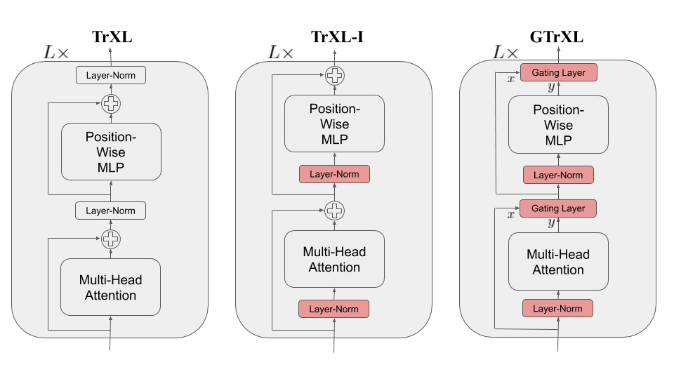
The first change is to place the layer normalization on only the input stream of the submodules. The model using this Identity Map Reordering is termed TrXL-I in the following, and is depicted visually in above Figure. A key benefit to this reordering is that it now enables an identity map from the input of the transformer at the first layer to the output of the transformer after the last layer.
3.2 Gating Layers
Further improve performance and optimization stability is achieved by replacing the residual connections in (9) with gating layers. The gated architecture with the identity map reordering is called the Gated Transformer(-XL) (GTrXL). The final GTrXL layer block is written below:
\[\overline Y^{(l)} = RelativeMultiHeadAttention(LayerNorm([StopGrad(M^{(l-1)}),E^{(l-1)}]))\] \[Y^{(l)} = g_{MHA}^{(l)}(E^{(l-1)},ReLU(\overline Y^{(l)})) \tag{10}\] \[\overline E^{(l)} = f^{(l)}(LayerNorm(Y^{(l)}))\] \[E^{(l)} = g_{MLP}^{(l)}(Y^{(l)},ReLU(\overline E^{(l)}))\]where g is a gating layer function. Here are a variety of gating layers with increasing expressivity:
Input: The gated input connection has a sigmoid modulation on the input stream:
\[g^{(l)}(x,y) = \sigma(W_{g}^{(l)}) \odot x + y \tag{11}\]Output: The gated output connection has a sigmoid modulation on the output stream:
\[g^{(l)}(x,y) = x + \sigma(W_{g}^{(l)} - b_{g}^{(l)}) \odot y \tag{12}\]Highway: The highway connection modulates both streams with a sigmoid:
\[g^{(l)}(x,y) =\sigma(W_{g}^{(l)} + b_{g}^{(l)}) \odot x + (1 - \sigma(W_{g}^{(l)} + b_{g}^{(l)})) \odot y \tag{13}\]Gated-Recurrent-Unit-type gating: The Gated Recurrent Unit (GRU) is a recurrent network that performs similarly to an LSTM but has fewer parameters:
\[r=\sigma\left(W_r^{(l)} y+U_r^{(l)} x\right), \quad z=\sigma\left(W_z^{(l)} y+U_z^{(l)} x-b_g^{(l)}\right), \quad \hat{h}=\tanh \left(W_g^{(l)} y+U_g^{(l)}(r \odot x)\right), \tag{14}\] \[g^{(l)}(x, y)=(1-z) \odot x+z \odot \hat{h} .\]IV. Code
(To be Continued!)
V. Conclusion
(To be Continued!)